
Science fiction is replete with faster-than-light (FTL) travel. Warp drives, hyperspace jumps, and wormholes are staples of interstellar narratives, fueling our imagination about traversing the vast cosmic distances. But does any of this have a basis in reality? For over a century, the consensus in physics has been a resounding no. Einstein’s theory of special relativity firmly established the speed of light as a cosmic speed limit, an insurmountable barrier for anything traveling through space. Yet, a deeper dive into fundamental physics, particularly within the framework of the Wolfram Physics Project, reveals a more nuanced and intriguing picture. Is faster-than-light travel truly an impossibility, or is it merely an extraordinarily complex engineering challenge? This exploration delves into the theoretical underpinnings of FTL possibilities, suggesting that breaking the light speed barrier might not be about defying physical laws, but rather about ingeniously “hacking” the very fabric of space.
 Faster than Light in Our Model of Physics: Some Preliminary Thoughts
Understanding Space and Time in Wolfram Physics
To grapple with the concept of faster-than-light travel, we must first reconsider our understanding of space and time. Traditional physics, rooted in general relativity, portrays space (and spacetime) as a smooth, continuous background – a manifold upon which the events of the universe unfold. In this view, every point in space can be described by three coordinate values, forming a seamless continuum. However, the Wolfram Physics Project proposes a radical departure from this classical picture. Space, in this model, is not merely a passive backdrop but possesses a definite, intrinsic structure. In fact, everything in the universe, from particles to forces, is ultimately conceived as emerging from this underlying spatial structure. At a fundamental level, everything is “made of space.”
Imagine water, which appears to be a continuous fluid at a macroscopic scale. Yet, we know that at a microscopic level, water is composed of discrete molecules. Similarly, the Wolfram model posits that space, at its most fundamental level, is also discrete, built from “atoms of space.” Only at larger scales does this discrete structure give rise to the continuous space we perceive.
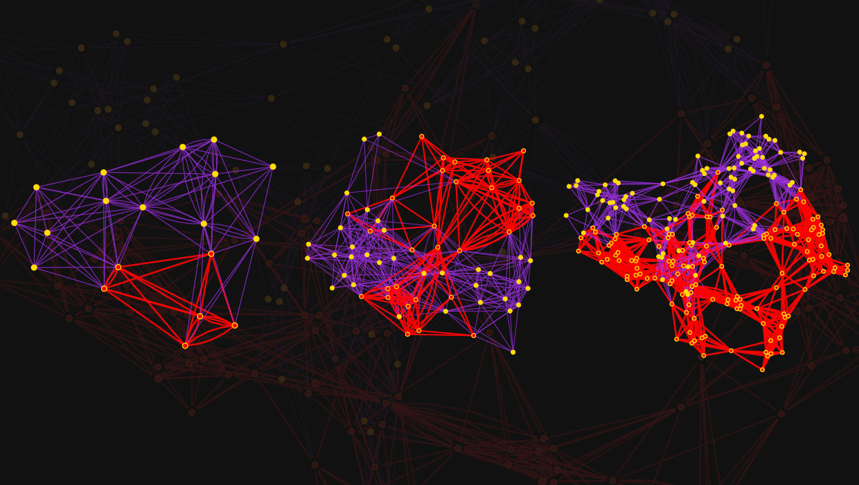
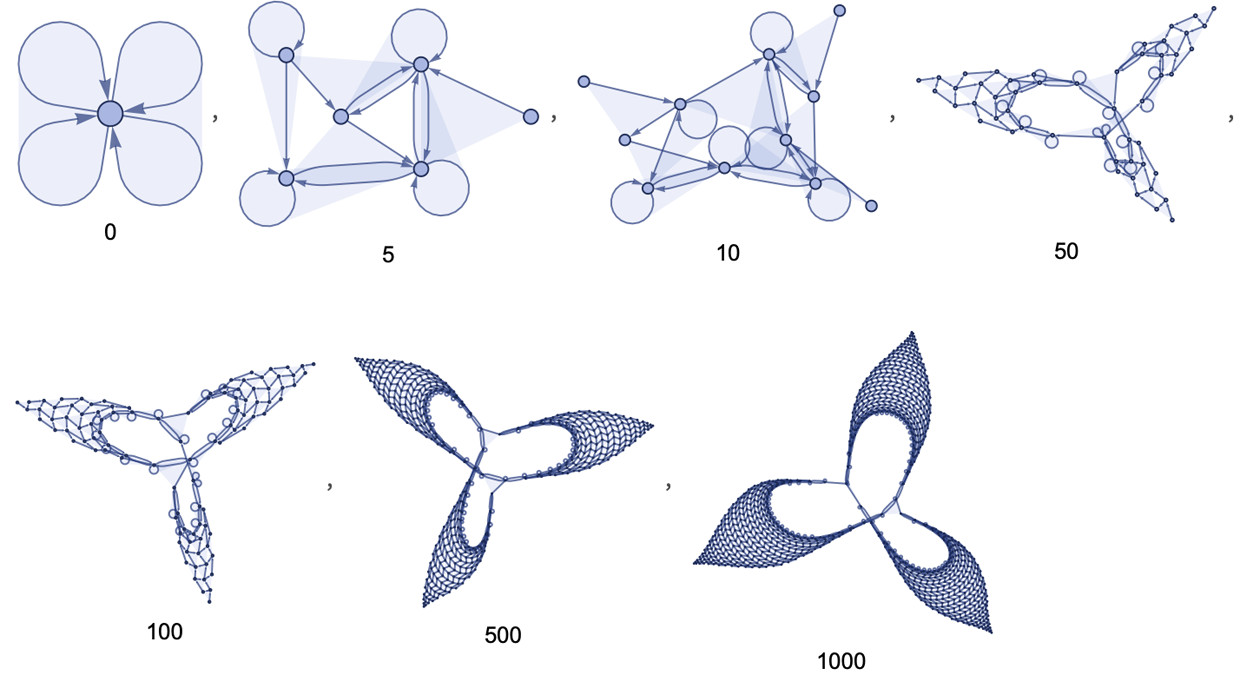
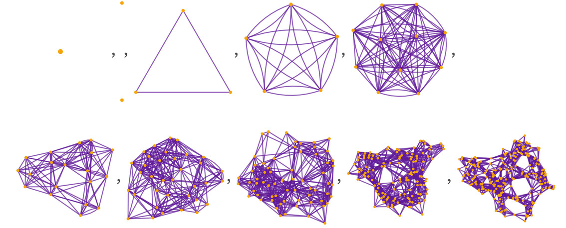
In this model, these “atoms of space” are not particles in space, but rather abstract elements defined solely by their relationships to other elements. Mathematically, this structure can be represented as a hypergraph, where the atoms of space are nodes, and their relationships are hyperedges connecting these nodes. At an extremely small scale, a snapshot of space might resemble a complex network of interconnected nodes.
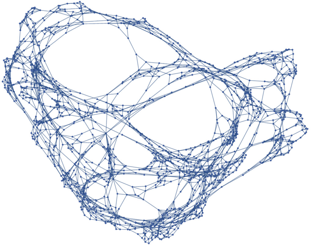
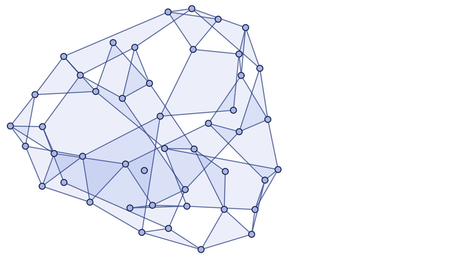
As we zoom out to slightly larger scales, the hypergraph might appear more structured.
 Graph3D
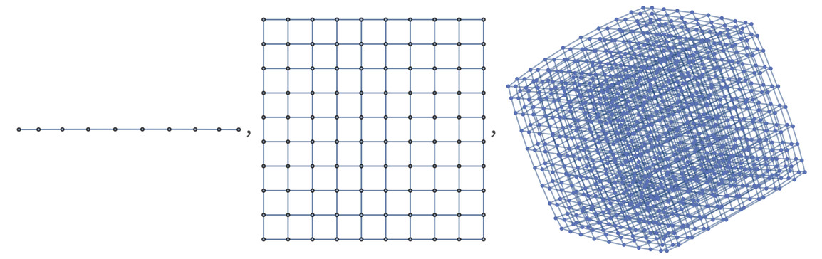
In our universe, this hypergraph is theorized to be incredibly vast, potentially containing around 10400 nodes. The dimensionality of space, in this framework, is not a predetermined constant but an emergent property. Different hypergraphs can exhibit different dimensional behaviors. Some might behave like 2D surfaces, while others might mimic 3D space, or even spaces with non-integer dimensions.
 Table
Table
The dimensionality is determined by how the number of nodes within a “geodesic ball” grows with its radius. A geodesic ball is defined as the region reachable by traversing at most r connections in the hypergraph. In a d-dimensional space, the number of nodes in a geodesic ball scales as rd. Curvature in space introduces corrections to this relationship.
Remarkably, the Wolfram model suggests that the large-scale, aggregate dynamics of these discrete spatial elements give rise to the properties of space described by Einstein’s equations of general relativity. This means that the familiar laws of gravity and spacetime curvature emerge from the underlying structure of the hypergraph.
But if space is this network of interconnected elements, what then is time? Unlike standard physics, time in this model is not a dimension on par with space. Instead, it is intrinsically linked to the process of computation that drives the evolution of the spatial hypergraph. Time arises from the sequential updating of the hypergraph’s structure according to a fundamental rule.
Consider a rule that dictates how local portions of the hypergraph are updated.
Applying this rule repeatedly leads to a sequence of hypergraph states.
 Flatten
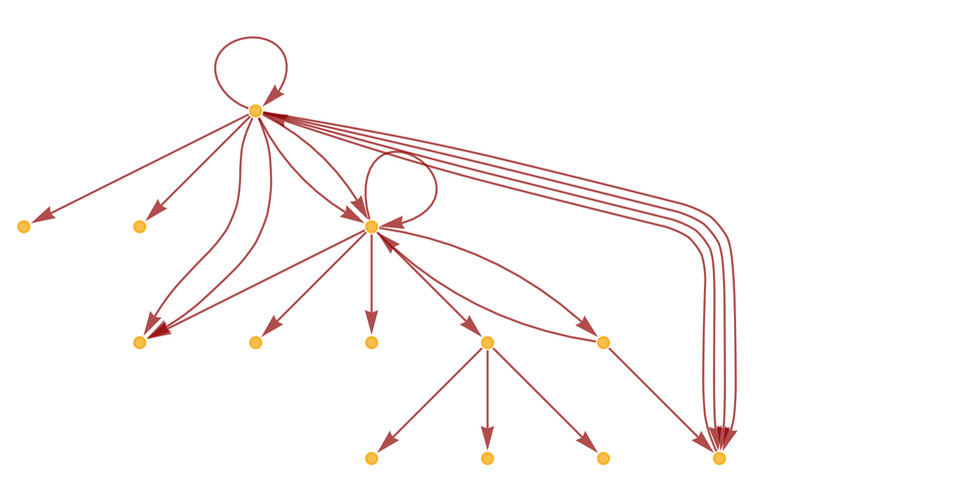
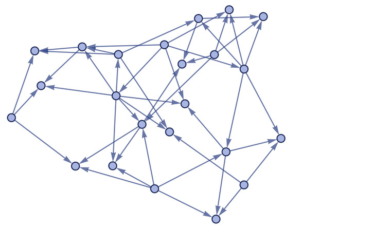
However, a crucial point is that the rule only specifies how updates occur, not when or where. If multiple regions of the hypergraph match the rule’s conditions, there’s no inherent order dictating which update happens first. This leads to the concept of a “causal graph,” which tracks the causal relationships between these updating events. An update can influence subsequent updates, creating a network of dependencies.
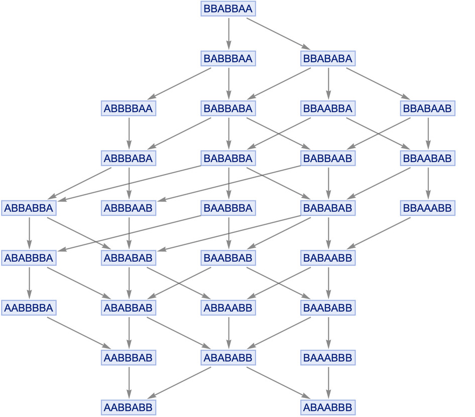
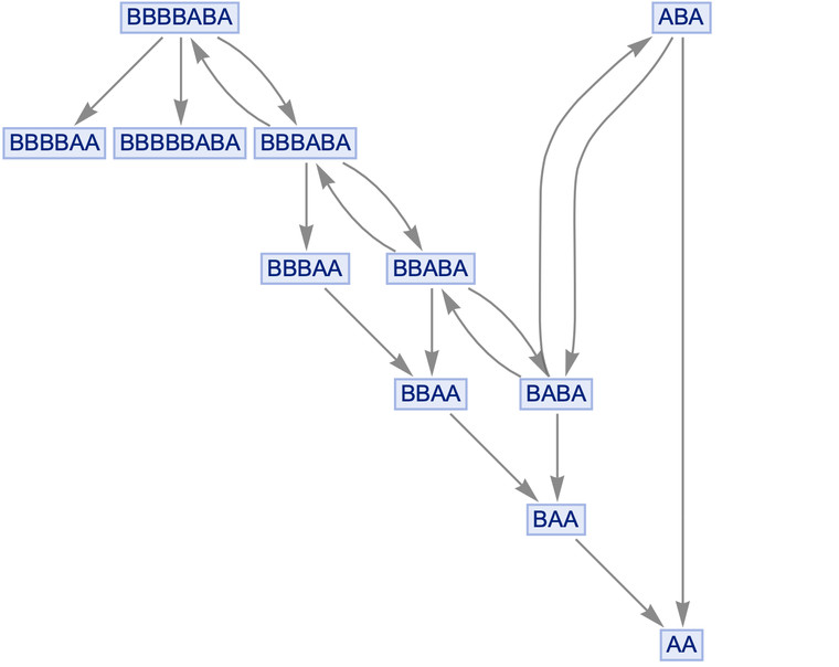
To visualize this more clearly, consider a simpler analogy using strings of characters. Imagine a rule that sorts characters in a string, like BA → AB. Applying this rule repeatedly to a string creates a sequence of updates.
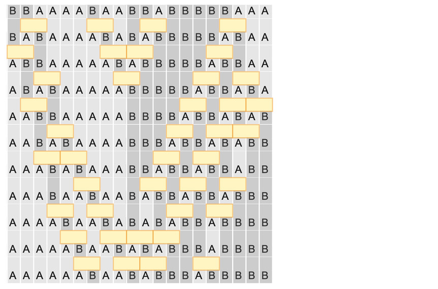 evo = (SeedRandom
The yellow boxes represent updating events, and we can connect them with a causal graph to show which events influence others.
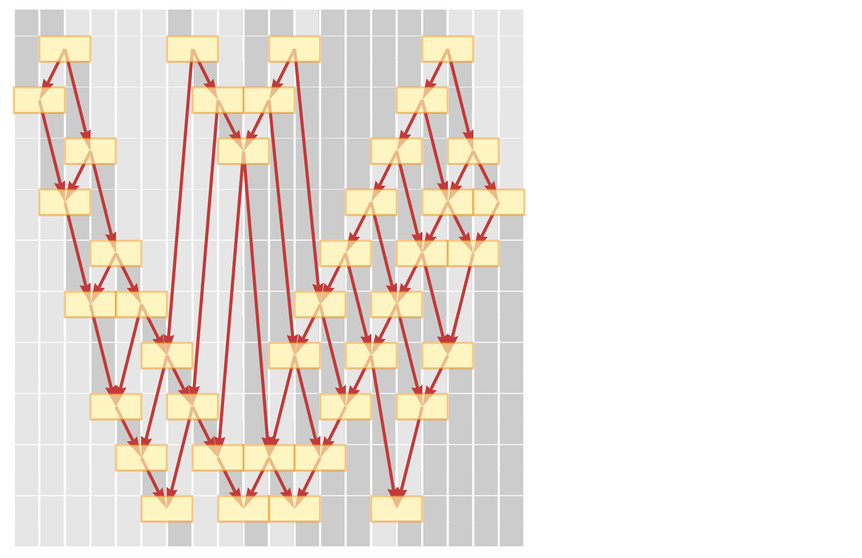 evo = (SeedRandom
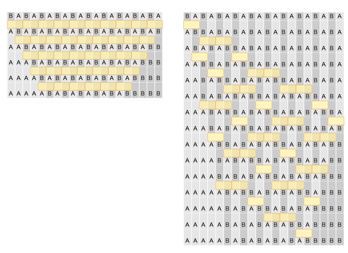
Within this system, an observer only perceives events and their causal connections. To describe this evolution, we introduce the idea of “simultaneity surfaces” or “reference frames,” allowing us to organize events in time.
Different choices of reference frames are possible.
These different reference frames are analogous to reference frames moving at different speeds in special relativity. The rule used in this string example exhibits “causal invariance,” meaning that the causal graph remains the same regardless of the order of updates. This causal invariance is key to deriving special relativity from this fundamentally different starting point where space and time are not initially the same.
From a causal graph and a chosen reference frame, we can reconstruct the system’s behavior.
 CloudGet
The apparent slowing down in the second reference frame reflects relativistic time dilation. Causal graphs can also be constructed for spatial hypergraphs, representing the causal relationships between updates in space.
 ResourceFunction
Reference frames can again be defined in these spatial causal graphs, with the constraint that each “slice” of simultaneity must be spacelike, containing no causally connected events.
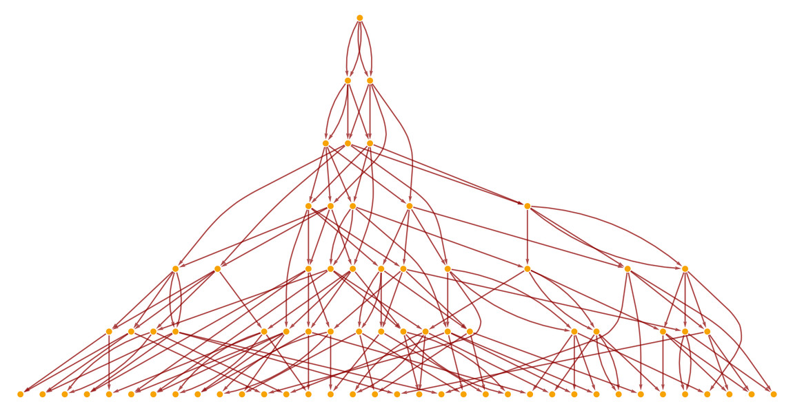
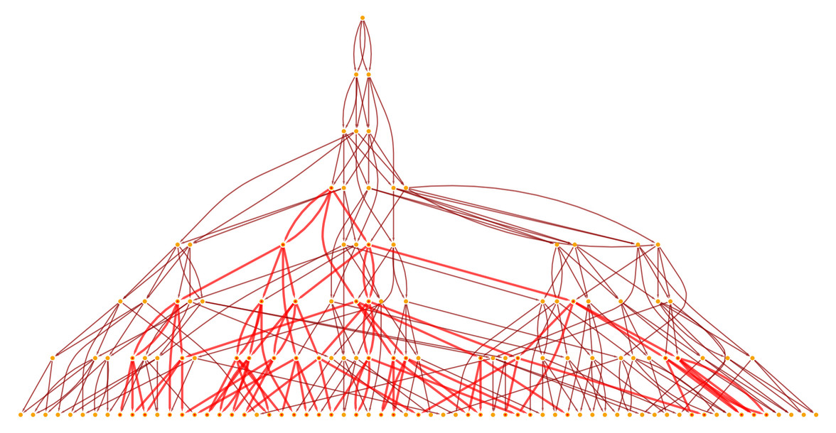
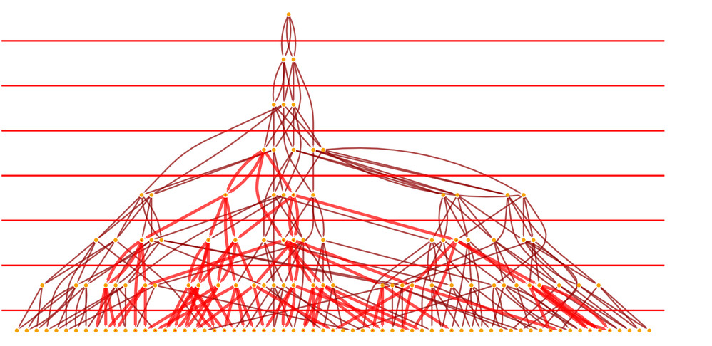
Beyond a single causal history, our models naturally lead to the concept of a “multiway graph,” encompassing all possible update orderings and histories of the system.
 LayeredGraphPlot
Each node in this multiway graph represents a complete state of the system, and paths through it represent possible evolutions, each with its own causal graph. The existence of this multiway graph is deeply connected to the emergence of quantum mechanics in these models. Just as reference frames help understand spacetime evolution, “quantum observation frames” help make sense of the multiway graph’s evolution. Analogous to physical space, “branchial space” emerges as a space of quantum states, with connections defined by relationships within the multiway system.
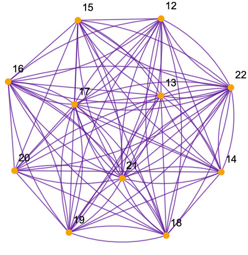
Branchial graphs can be constructed to represent relationships between quantum states in branchial space, much like spatial hypergraphs represent spatial relationships.
Just as Einstein’s equations describe the large-scale behavior of spatial hypergraphs, the large-scale behavior of multiway systems seems to give rise to Feynman’s path integral formulation of quantum mechanics. Furthermore, similar to the speed of light c limiting motion in physical space, a maximal entanglement rate ζ limits exploration and entanglement in branchial space. This sets the stage for considering not only “faster than light” but also “faster than ζ” phenomena.
Space Tunnels and Wormholes: Shortcuts Through Spacetime
General relativity depicts space as a continuous manifold, but our models reveal a discrete, underlying structure. While our models can reproduce general relativity in appropriate limits, they also suggest novel phenomena beyond its scope, including the intriguing possibility of space tunnels.
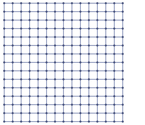
Imagine a spatial hypergraph resembling a simple 2D grid.
 GridGraph
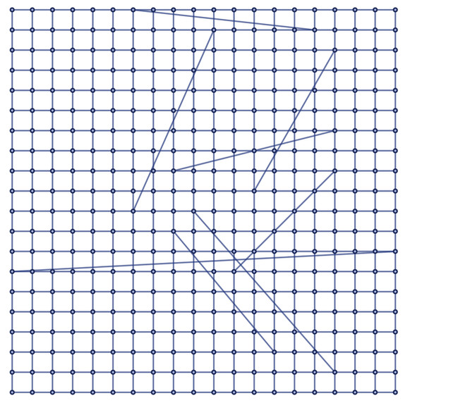
This grid approximates 2D Euclidean space. Now, introduce “long-range threads” – extra connections bridging distant parts of the grid.
 SeedRandom
This modified graph can also be rendered in 3D to better visualize the shortcuts.
The presence of these long-range threads dramatically alters distances within the graph. Some nodes remain at expected distances as in ordinary 2D space, but others become “anomalously close” due to these shortcuts. Traveling along these threads allows bypassing the usual spatial distances.
If we consider movement as traversing one connection in the hypergraph per unit time, these long-range threads effectively create “space tunnels” allowing faster transit between distant spatial locations than would be possible through ordinary space. These tunnels can be persistent, allowing repeated use, or transient, appearing spontaneously and briefly.
Space tunnels, in this general sense, can manifest in various forms within graphs and hypergraphs. A specific realization within general relativity is the wormhole. Wormholes, in continuous spacetime, are conceptual “handles” connecting different regions, offering alternative paths.
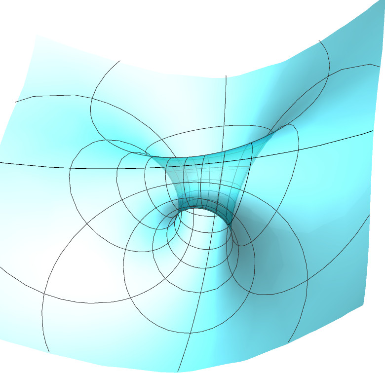 Wormhole diagram
Image alt text: Diagram of a wormhole, illustrating it as a shortcut connecting two distant regions of spacetime.
How such topologically complex manifolds form within general relativity is a challenge, often invoking singularities. However, in our discrete models, topology change becomes more natural. Instead of continuously deforming a manifold, we can envision “growing a handle thread by thread” in the hypergraph.
Consider a rule that effectively “knits handles” in patches of hypergraph that approximate 2D Euclidean space.
 Labeled
Freed from the constraints of continuity, space in our models can exhibit exotic geometries. Dimension itself becomes a dynamical variable, not fixed to integer values. Regions of space can have varying dimensionality. For example, a hypergraph approximating 2.3-dimensional space.
 ResourceFunction
Space tunnels, therefore, can manifest as regions of altered dimensionality. Lower-dimensional tunnels (like extended 1D threads) could connect sparsely distributed distant points. Higher-dimensional tunnels (approaching tree-like structures in the infinite dimension limit) could act as “switching stations,” bringing numerous boundary points closer together. Both types offer intriguing possibilities for circumventing normal spatial distances.
Negative Mass and Maintaining Space Tunnels
Once a space tunnel, particularly a wormhole-like structure, is formed, the question of its stability arises. General relativity suggests maintaining wormholes is challenging due to the evolution of spacetime governed by Einstein’s equations. Wormholes are characterized by converging geodesics at entry and diverging geodesics at exit. Gravity, associated with mass, typically causes geodesics to converge. To achieve divergence, some form of gravitational repulsion is needed, which, in general relativity, points towards the necessity of negative mass.
Mass is typically considered a positive quantity, but concepts like dark energy effectively require negative mass. Several phenomena in traditional physics hint at effective negative mass scenarios, often related to the zero-point energy of the vacuum. The vacuum, even in classical physics, is not truly empty but is thought to be filled with fields like the Higgs field and quantum vacuum fluctuations, each contributing to energy density.
Normally, we set the zero point of energy to include these universal vacuum contributions. However, if something could locally reduce these vacuum effects, it could manifest as negative mass relative to the “normal vacuum.” The Casimir effect, where confining vacuum within a box restricts certain quantum field fluctuations, leading to a measurable negative energy density inside the box compared to the outside vacuum, is an example. However, extrapolating Casimir effects into a purely gravitational or spacetime context is complex.
In our models, the vacuum is not simply empty space but a structured state of the hypergraph itself. Vacuum fluctuations and other quantum field phenomena are not happening in space but are integral to the very formation of space. Space, matter, particles, and quantum fields are all manifestations of the hypergraph’s structure.
Energy in our models is related to the rate of updating activity in the hypergraph. A region with reduced updating activity would have negative energy relative to the “normal vacuum.” We can conceptually call something that reduces hypergraph activity a “vacuum cleaner.” If such “vacuum cleaners” could exist, they could potentially create and maintain wormholes, as regions with reduced activity would cause geodesics to diverge.
While large-scale wormholes likely require negative mass and vacuum cleaners, other types of space tunnels might not have the same stringent requirements. Their very nature, often operating outside the regime smoothly described by general relativity, means standard singularity theorems may not apply. Analyzing their behavior requires direct investigation within the framework of our discrete models.
A tempting approach would be to simulate space tunnel configurations to assess their stability. However, computational irreducibility poses a significant challenge. Simulations might show stability for limited steps, but long-term stability, relevant to human timescales, might be computationally undecidable. Even if engineered, maintaining a space tunnel might require ongoing, potentially infinite, “engineering tweaks,” and ultimate stability cannot be guaranteed. The first step, however, remains to understand how to construct a space tunnel in the first place.
Faster Than Light, Not Time Travel
General relativity, often treating spacetime as a unified entity, raises the specter of time travel when considering wormholes. If a wormhole connects two spatial locations, it might also seem to connect different moments in time. A shortcut through time could lead to scenarios where the future influences the past, potentially creating paradoxes.
While future-to-past causality might seem paradoxical, it’s not entirely foreign. Periodic systems, for example, exhibit a future that is a repetition of the past. However, this is a predetermined future, not one we can freely alter.
In standard general relativity, the mathematical formalism becomes complex when considering wormholes and time travel. Consistent solutions to Einstein’s equations in such scenarios might require locking past and future into something akin to periodic behavior. The idea of “motion in time” arises from treating time as just another coordinate in spacetime.
However, in our models, space and time are fundamentally distinct. Space emerges from the spatial hypergraph’s structure, while time is rooted in the computational process of updates. This computational process is inherently computationally irreducible.
While spatial exploration within the hypergraph is conceivable, temporal progression is tied to the irreversible computation of the universe. We can compute future states (or, with limitations, past states), but only by effectively enacting the computational steps. We cannot “move through time” separately to observe past or future states.
Causality is explicitly tracked and represented by the causal graph.
Crucially, causal graphs in our models are acyclic; they contain no loops. There’s a clear “flow of causality,” a partial ordering of events without feedback loops where an event affects itself.
Different “simultaneity surfaces,” representing reference frames, can be defined within the causal graph.
But these foliations always maintain a consistent “causally forward” progression of time. Causal invariance, a property of many rules in our models, ensures this consistent temporal directionality.
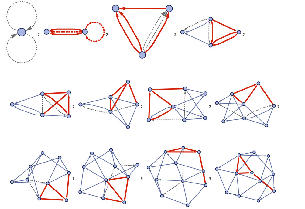
Breaking causal invariance can lead to different behaviors. Consider a multiway system with a rule lacking causal invariance. The multiway graph might exhibit loops, revisiting the same state repeatedly.
 Graph
Graph
The corresponding multiway causal graph in such systems can contain loops, representing closed timelike curves – scenarios where the future can influence the past.
 LayeredGraphPlot
In general relativity, such loops are associated with time travel. However, these time loops are distinct from space tunnels. Space tunnels provide spatial connectivity, shortening spatial distances, but don’t inherently violate the forward progression of time. Events at either end of a space tunnel, while spatially distant in ordinary space, remain temporally ordered according to the causal graph, respecting causality. “Jumping” between distant spatial locations via a space tunnel does not necessitate or imply “traveling backwards in time.” While flat, continuum spacetime might imply time reversal for tachyons exceeding light speed, the existence of space tunnels fundamentally alters this picture. Time, as a computational progression, can continue forward even as effects propagate faster than light through space tunnels, connecting spatially distant regions.
Causal Cones, Light Cones, and Spatial Distance
Let’s now delve into the core question of faster-than-light effects in our models. When an event occurs, it influences a cone of subsequent events in the causal graph – its causal cone. In a simple grid-like causal graph, this is straightforward.
 CloudGet
However, in more realistic causal graphs derived from our models, the structure is more complex.
 With
With
The causal cone, representing the domain of influence, remains well-defined. But how does this relate to space and time as we perceive them? In spacetime, we often think of light cones – the region in spacetime reachable by light emitted from a point. One might naively assume causal cones and light cones are identical. However, this is a subtle point. Light cones are defined by spatial and temporal positions, which are readily available in continuous spacetime manifolds. In our models, however, positions in space are not intrinsic. We can identify affected hypergraph elements after a sequence of events, but their spatial location is not a priori defined. Spatial location emerges in a large-scale limit, relative to the overall hypergraph structure.
This is the crux of faster-than-light effects in our models: causal relationships are fundamental and immediate, while spatial relationships are emergent. An event can influence another through a single causal link, even if these events are at opposite ends of a space tunnel, seemingly separated by vast spatial distances.
Several interconnected issues arise, all revolving around the nature of space in our models. We began by defining space through hypergraphs, but these hypergraphs are dynamic, constantly evolving. Can we even define an instantaneous snapshot of space?
Reference frames, foliations, and simultaneity surfaces provide a way to define such snapshots. They specify a collection of events considered to occur “at the same time,” allowing us to sample the spatial structure. This choice is not unique, reflecting the reference frame dependence inherent in relativity.
Can we choose any collection of events consistent with the causal ordering (where no events in a “time slice” are causally related)? This is where complexity deepens. Consider a highly irregular foliation.
 CloudGet
While we might have a sense of the “typical” spatial hypergraph structure, with a sufficiently convoluted foliation, the instantaneous spatial structure could become drastically different.
For now, let’s assume a “reasonable” foliation. We then ask: what is the “projection” of the causal cone onto this instantaneous spatial structure? In other words, which spatial elements are affected by a given event?
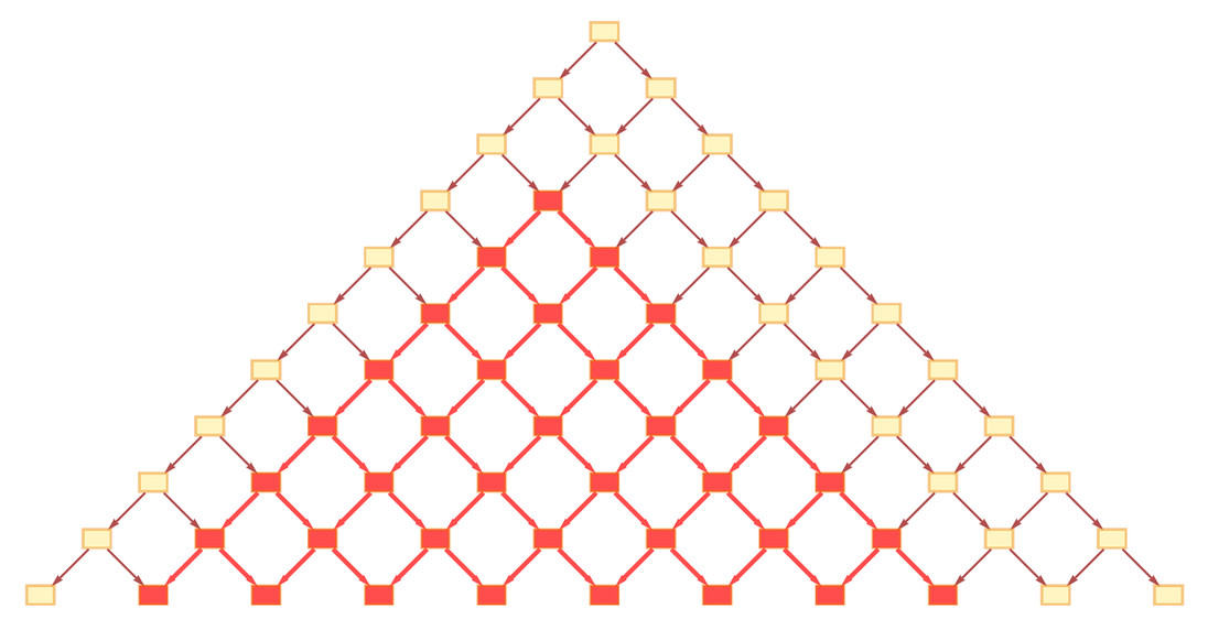
Consider the same rule and causal cone as before, using a “flat” foliation (corresponding to a “cosmological rest frame”).
CloudGet
Now examine the spatial hypergraphs associated with successive slices of this foliation, highlighting the portions within the causal cone.
 alt
alt
For the initial slices, the initiating event is yet to occur. Subsequently, the effect of the event propagates, expanding across spatial hypergraphs in successive slices. This visualization depicts the expansion of a light cone over time. The crucial question now is: what is the speed of this expansion? How much spatial distance is traversed per unit time? This defines the effective speed of light within the model.
From these images, it’s evident this is not a straightforward question. Let’s consider a more fundamental issue. The speed of light is measured in units like meters per second. Our model, however, might initially give us a speed in hypergraph edges per causal edge. Each causal edge represents an elementary time step. Defining a “second” effectively scales elementary time steps to seconds. Similarly, spatial hypergraph edges can be scaled to elementary lengths, defining “meters.” If the light cone advances by α spatial hypergraph edges in t elementary time steps, then the spatial advance in meters is α c t, where c is the speed of light. Therefore, the speed of light is, in a sense, defined by the rate of expansion of the light cone in the spatial hypergraph.
However, unlike continuum space with a constant speed of light in all directions, projecting a causal cone onto a spatial hypergraph makes this less straightforward. The speed of light may not be uniform in all “directions” within the hypergraph. Characterizing space and distance becomes crucial to precisely define and measure speed in this context. While causal effects and their propagation are well-defined, their precise manifestation in what we perceive as space requires further investigation. We understand causal cones, but how they map to spatial positions, and whether this allows for effects exceeding the speed of light relative to our spatial framework, remains to be fully elucidated.
Measuring Distance in Hypergraphs
Speeds are challenging to define in our models because positions and times themselves require careful definition. Consider a simpler case: cellular automata, where space and time are inherently discrete grids. In cellular automata, we can ask: how fast can an effect propagate? If we alter a single cell’s initial state, how many cells per time step does this perturbation spread?
Here are examples of cellular automata evolutions.
Image alt text: Evolutions of two cellular automata rules (Rule 22 and Rule 30), showing the propagation of changes from an initial perturbation.
The expansion speed varies, but the maximum speed is 1 cell per step in both cases. This is directly understandable from the rules themselves.
Image alt text: Rule diagrams for cellular automata Rule 22 and Rule 30, illustrating the local neighborhood of influence for each rule.
Both rules affect cells within a radius of one cell per step, thus limiting the maximum propagation speed to 1 cell/step. A similar principle applies to our models. Rules, like:
only “reach” a limited number of connections away. Each update event affects elements within a limited hypergraph distance. However, the global spatial structure is not predefined as in cellular automata. The local nature of rules does not immediately dictate global speed limits because the “relative geometry” of successive updates and connections is dynamically determined.
Rules can even be non-local. If the rule’s left-hand side is disconnected.
then an update can potentially connect elements from anywhere in the hypergraph, even disconnected parts. This could lead to instantaneous effects across the “universe,” but such rules might not generate the locality properties characteristic of space as we know it.
Given a spatial hypergraph, how do we quantify “distance” between nodes? Graph distance – the length of the shortest path – is straightforward to compute. However, this is an abstract hypergraph distance. How does it relate to physical distance, measurable with a “ruler”?
This is a subtle issue. We have a hypergraph representing the universe, and we want to use something within this hypergraph, presumably, to measure distance within it. Traditional relativity uses light signals for distance measurement, implicitly assuming a pre-existing spatial structure. In our models, photons themselves must emerge from the hypergraph structure. They are “pieces of space” with specific topological properties.
When directly examining spatial hypergraphs, we are operating far below the level of photons. To compare hypergraph distances to physical distances, we need a bridge – a proxy for physical distance computable directly within the hypergraph.
A simple proxy is graph distance, with a refinement. Hypergraph relations are ordered (directed hyperedges). For “physical-like distances,” we can ignore directionality and treat the hypergraph as undirected. For large hypergraphs, this approximation should be reasonable, although directedness might relate to spinors, while undirectedness corresponds to vectors, more familiar in distance measurements.
Are there other distance proxies? Yes, several, including one derived from the causal graph itself, analogous to a “branchial distance for the causal graph.” This is akin to relativity discussions using beacons signaling over time. In our model, it’s analogous to a branchial distance in the causal graph.
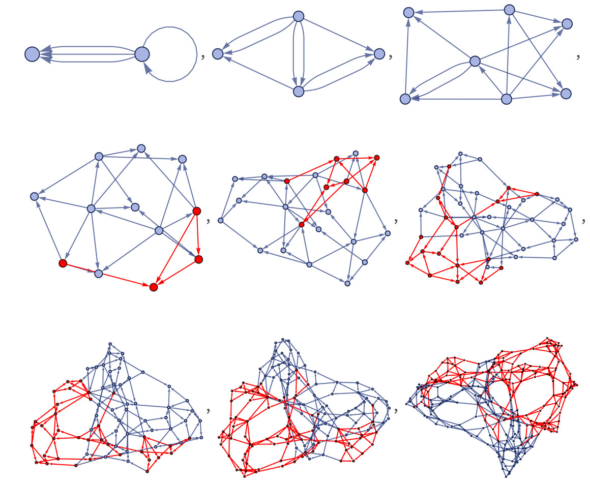
Here’s how it works: construct a causal graph.
Consider events in the last slice. For each pair, examine their ancestry – previous events leading to them. If a pair shares a common ancestor in the preceding step, connect them. This yields a “spatial reconstruction graph.”
 SpatialReconstruction
In an appropriate limit, this should approximate the original spatial hypergraph structure, although for small graphs, differences are noticeable.
 ResourceFunction
It’s crucial to distinguish between these graphs. The spatial hypergraph’s nodes are fundamental “atoms of space,” and hyperedges represent relations. Causal graph nodes are updating events, with edges representing causal dependencies. The spatial reconstruction graph has events as nodes, but edges represent immediate common ancestry – events in the same “elementary light cone.” A causal graph knits together these elementary light cones. The spatial reconstruction graph infers proximity between events based on their shared elementary light cone.
There’s an analogy to quantum mechanics. In quantum mechanics, multiway graphs have quantum states as nodes. “Branchial graphs” are constructed from slices, connecting states with immediate common ancestors in the multiway graph – states in the same “entanglement cone.” Branchial graphs map quantum state space and entanglements.
The spatial reconstruction graph is analogous – a branchial graph from the causal graph. (Edges in spatial reconstruction graphs are colored purple, a blend of “branchial pink” and spatial hypergraph blue-gray.)
In the spatial reconstruction graph above, edges connect events with common ancestors one step back. Generalizing this to ancestors more than one step back is possible. Going two steps back for the same example causes almost all events to share common ancestors.
 SpatialReconstruction
With sufficient lookback, all events will share the “big bang” event as a common ancestor. Consider a rule generating spatial hypergraph sequences.
 ResourceFunction
Compare these to spatial reconstruction graphs from this system’s causal graph, with a 2-step lookback.
ResourceFunction
As steps increase, spatial hypergraphs and spatial reconstruction graphs exhibit growing similarity, though not identical. Spatial reconstruction graphs are not the only distance proxy. Common successors instead of ancestors could be used. Another option is to consider “dual spatial hypergraphs,” where nodes represent relations and hyperedges represent shared elements.
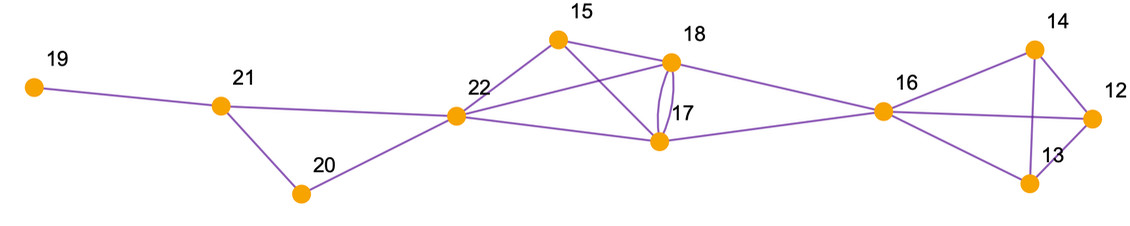
For the spatial hypergraph:
the dual spatial hypergraph is:
 UnorderedHypergraphPlot
The sequence of dual spatial hypergraphs for the earlier evolution is:
![Cell[CellGroupData[{Cell[BoxData[ RowBox[{ RowBox[{“RelationsElementsHypergraph”, “[“, “wmo“, “]”}], “:=”, RowBox[{“Module”, “[“, RowBox[{ RowBox[{“{“, RowBox[{ RowBox[{“ix”, “=”, RowBox[{“wmo”, “[“, RowBox[{“”””, “,”, RowBox[{“-“, “1”}]}], “]”}]}], “,”, “es”}], “}”}], “,”, RowBox[{“Values”, “[“, RowBox[{“Merge”, “[“, Rowbox[{ Rowbox[{“Association”, “@@@”, RowBox[{“(“, RowBox[{“Thread”, “/@”, RowBox[{“Thread”, “[“, RowBox[{ RowBox[{ RowBox[{“wmo”, “[“, “”””, “]”}], “[“, RowBox[{“[“, “ix”, “]”}], “]”}], “[Rule]”, “ix”}], “]”}]}], “)”}]}], “,”, “Identity”}], “]”}], “]”}]}], “]”}]}]], “Input”], Cell[BoxData[ RowBox[{ RowBox[{“UnorderedHypergraphPlot”, “[“, RowBox[{“h“, “,”, “opts___”}], “]”}], “:=”, RowBox[{ RowBox[{“ResourceFunction”, “[“, “”””, “]”}], “[“, RowBox[{“h”, “,”, “opts”, “,”, RowBox[{“”””, “[Rule]”, “0”}], “,”, RowBox[{“EdgeStyle”, “[Rule]”, RowBox[{“”}]}], “,”, RowBox[{“”””, “[Rule]”, RowBox[{“”}]}]}], “]”}]}]], “Input”], Cell[BoxData[ RowBox[{“UnorderedHypergraphPlot”, “[“, RowBox[{“RelationsElementsHypergraph”, “[“, RowBox[{ RowBox[{ “ResourceFunction”, “[“, “”””, “]”}], “[“, RowBox[{ RowBox[{“{“, RowBox[{ RowBox[{“{“, RowBox[{ RowBox[{“{“, RowBox[{“x”, “,”, “y”}], “}”}], “,”, RowBox[{“{“, RowBox[{“x”, “,”, “z”}], “}”}]}], “}”}], “[Rule]”, RowBox[{“{“, RowBox[{ RowBox[{“{“, RowBox[{“x”, “,”, “z”}], “}”}], “,”, RowBox[{“{“, RowBox[{“x”, “,”, “w”}], “}”}], “,”, RowBox[{“{“, RowBox[{“y”, “,”, “w”}], “}”}], “,”, RowBox[{“{“, RowBox[{“z”, “,”, “w”}], “}”}]}], “}”}]}], “}”}], “,”, RowBox[{“{“, RowBox[{ RowBox[{“{“, RowBox[{“0”, “,”, “0”}], “}”}], “,”, RowBox[{“{“, RowBox[{“0”, “,”, “0”}], “}”}]}], “}”}], “,”, “5”}], “]”}], “]”}], “]”}]], “Input”] }, Open ]]